Four types of crime data (i.e., residential break and enter crimes, commercial break and enter crimes, car thefts, and robberies) were obtained from Ottawa Police Department. Several spatial analyses were conducted in CrimeStat to study the spatial distribution of crimes.
To better visualize the residential crime spatial distribution, check out the interactive map.
Nearest neighbor analysis
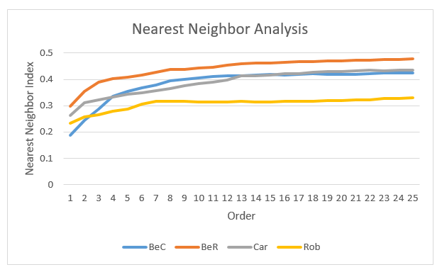
The nearest neighbor index of 1 indicates that the spatial distribution of points is completely random (CrimeStat, n.d.). Since the first order crimes of all these crime types had indices smaller than 0.5 indicating that they were more spatially aggregated than expected on the basis of chance.
The index changed as a function of the type of the crime as well as the nearest neighbor order. As the nearest neighbor order increased, the indices of all four crimes increased indicating that the crimes were more dispersed and closed to a random distribution.
Residential break and enter crimes were less spatially aggregated than commercial break and enter crimes for all the 25 orders. Car thefts were less spatially aggregated than robberies for all the 25 orders. While residential break and enter crimes were the lease spatially clustered for different orders, the spatial clustering of commercial break and enter crimes became smaller than car thefts and robberies after the 4th order. Generally, robberies tended to be the most spatially aggregated, while residential break and enter crimes tended to be the least spatially aggregated. Based on the land use map, residence areas were large and across the whole city which may lead to more dispersed distribution of residential crimes. However, commercial areas were restricted at certain locations, thus, commercial crimes were more clustered especially when the nearest neighbor order was small and crimes happened within one commercial area. Similarly, robberies and car thefts tended to happen within certain areas.
Moran's I analysis
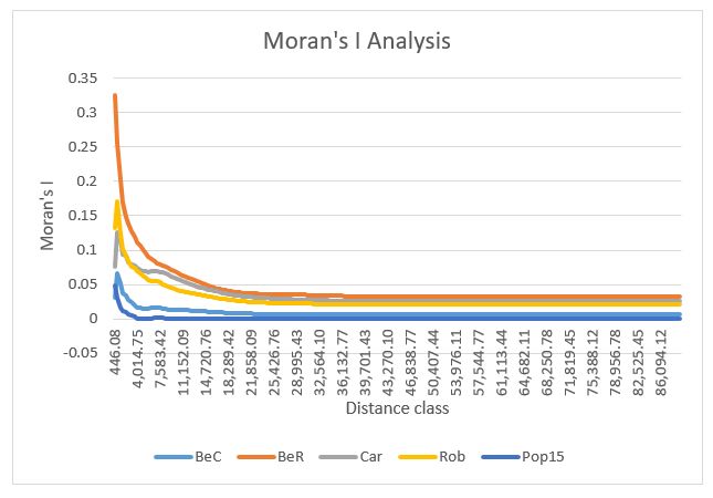
The Moran’s I of 0 indicates that the spatial distribution of points is completely random (CrimeStat, n.d.). With the increase in distance, Moran’s I of population data approached 0 indicating that population was randomly distributed, while the other intensity variables were spatially aggregated (CrimeStat, n.d.). Residential crimes were the least clustered, followed by commercial crimes. Robberies were the most clustered and car thefts ranked the 2nd most clustered.
Although both analyses showed that the four crimes were spatially clustered, the orders of the degree of clustering were different. In the nearest neighbor analyses, robberies were the most aggregated while commercial crimes were the most aggregated in Moran’s I analysis.
Moran’s I values of population decreased to 0 with the increase in distance (CrimeStat, n.d.). The distribution of population can be considered as completely random at the global level. As a result, population should be the “default”. Crimes were not distributed simply based on the population distribution because their Moran’s values were not equal to that of the population values. Therefore, all types of crimes showed spatial autocorrelation.
The comparison between the fuzzy mode (visual) clusters and the nearest neighbor hierarchical spatial clustering results
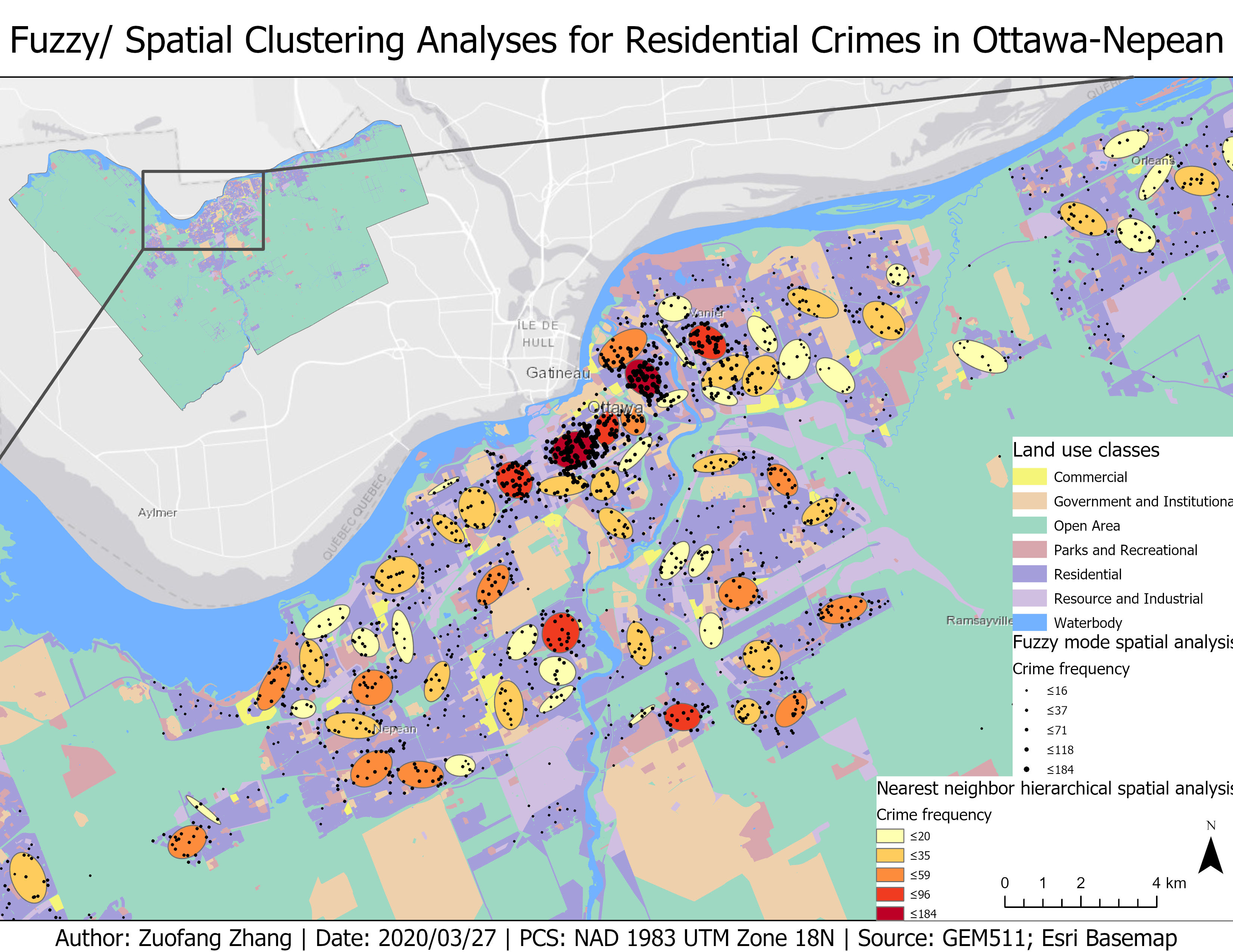
The fuzzy mode analysis uses the number of incidents occurring at different locations to identify hot spots where the number of crimes is the largest (CrimeStat, n.d.). The fuzzy mode result demonstrated the frequency of residential crimes in Ottawa-Nepean region. As shown in Fig.3, bigger the symbol, higher the frequency of crimes within 750m radius of a location. Most of the crime hot spots (i.e., locations with crime frequency bigger than 118) were in the central part of the city given the fuzzy mode result.
As opposed to the fuzzy mode which uses individual incidents to identify crime hot spots, the nearest neighbor hierarchical clustering analysis groups incidents that are spatially close (i.e., the distance threshold is 750m in this case) into clusters (CrimeStat, n.d.). The clusters were shown as ellipses in Fig.3 with darker red representing higher crime frequency. Generally, the two analyses gave the similar results that more crimes occurred in the central part of the city. However, the ellipses did not cover all incidents due to the restricted shape. Additionally, because the same crime incident may fall in multiple search radiuses around different locations, it may be counted multiple times leading to potential distortions. Therefore, the fuzzy mode result may be different from the nearest neighbor hierarchical spatial clustering analysis result.
The differences between the standard nearest neighbor hierarchical spatial clustering results and the risk-adjusted results
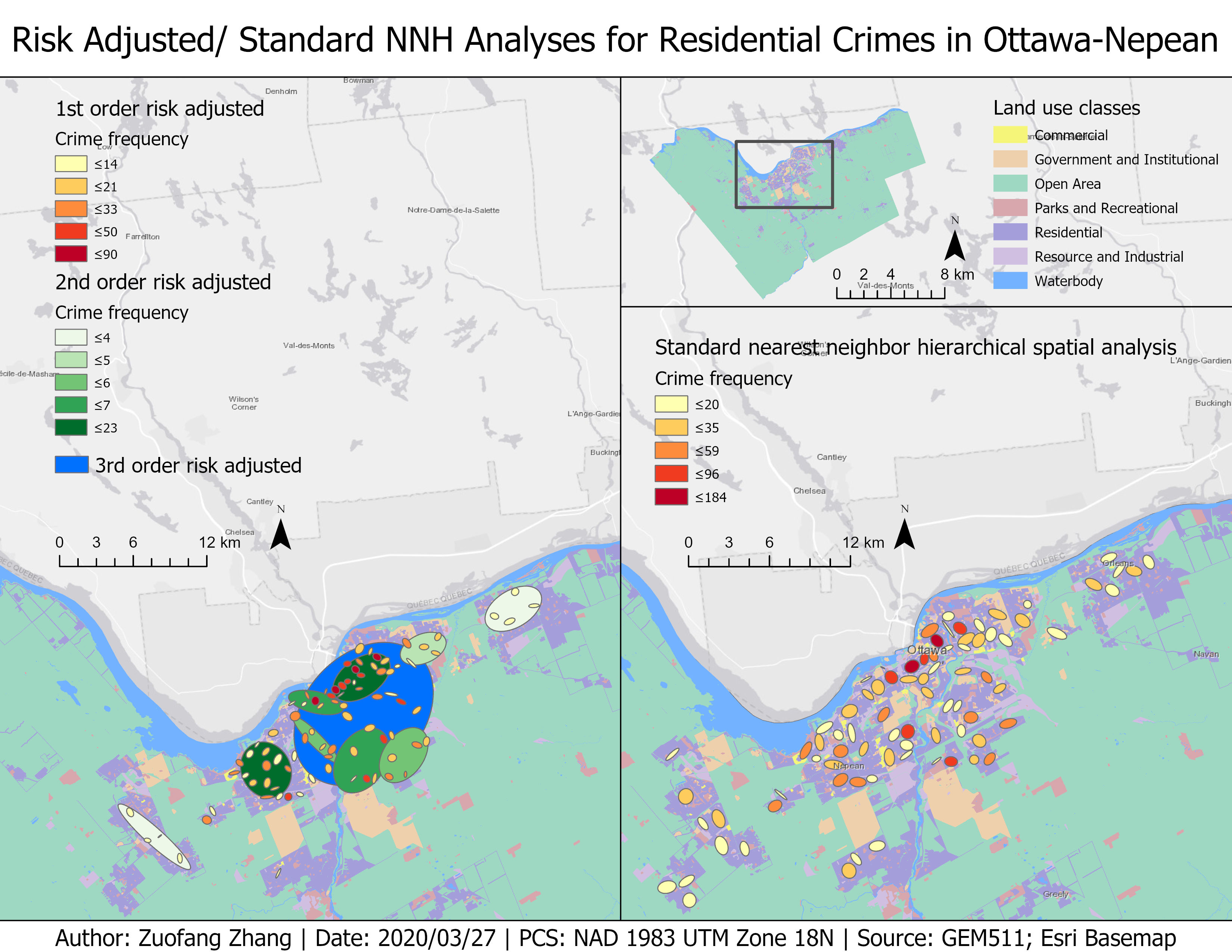
The risk-adjusted results considered the impacts of population of age 15 and above because this group of people was more often to be involved in or committed crimes. With different number of people showing up in a certain area, the number of crimes may be different. For example, crime clusters may relate to high concentration of population. Therefore, it is necessary to account for the difference in population and adjust the calculation accordingly. The risk-adjusted spatial clustering analysis uses not only a distance threshold but also a population baseline which makes it different from the standard NNH analysis (CrimeStat, n.d.). As shown in the left part of Fig.4, darker the color of ellipses are, higher risk of crimes occur within those ellipses.
The comparison of the 1st order results of both standard and risk-adjusted spatial clustering analyses showed that more crimes occurred in the central part of the city. However, the size of ellipses of risk-adjusted analysis was smaller than those of the standard results. This may due to the slightly different representations of the ellipses. The ellipses of the standard NNH referred to spatial clusters of crimes with different density or frequency, while those of the risk-adjusted NNH referred to crime clusters that were more aggregated than estimations on the basis of the population distribution. Additionally, in this case, the risk-adjusted NNH had three orders. The 1st order clusters was made based on individual incidents, which were then grouped into 2nd order clusters. The 2nd order clusters converged into a single big cluster in the end located in the central part of the city. The higher order clusters showed the relationship among several smaller lower order clusters. In other words, crime clusters tended to locate close to other crime clusters. Therefore, the 3rd order cluster included most of the lower order clusters.
A discussion on the results of the kernel density estimation
The kernel density approach was used to interpolate crime density over the entire study area. The fuzzy mode and NNH analyses studied the spatial distribution of the crime data themselves, while the kernel density approach generalized the data and made crime density estimations for the other part of the area (CrimeStat, n.d.). Additionally, the fuzzy mode and NNH analyses resulted in crime clusters represented by ellipses, while the kernel density estimation provided a continuous surface demonstrating crime density (CrimeStat, n.d.).
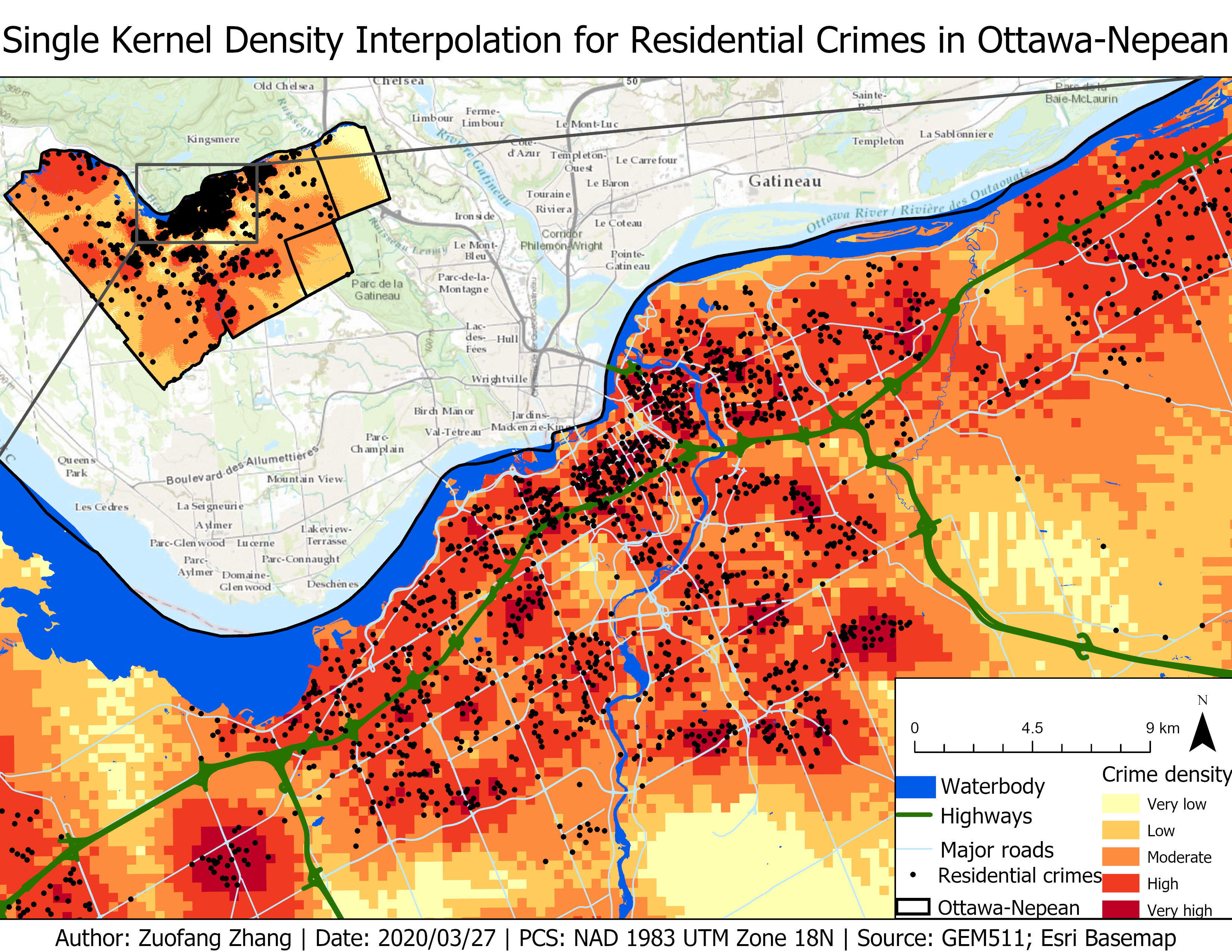
Fig.5 showed the residential crime density calculated using the single kernel density analysis with the incident locations overlaid on the top of the interpolation surface. Darker red indicated higher crime density and areas with higher crime density were located in the center part of the city as well as the northwest corner and the southeast corner of the Ottawa-Nepean region. However, residential crime observations were mainly clustered in the central part of the region, while only few of incidents were recorded in the surrounding area.
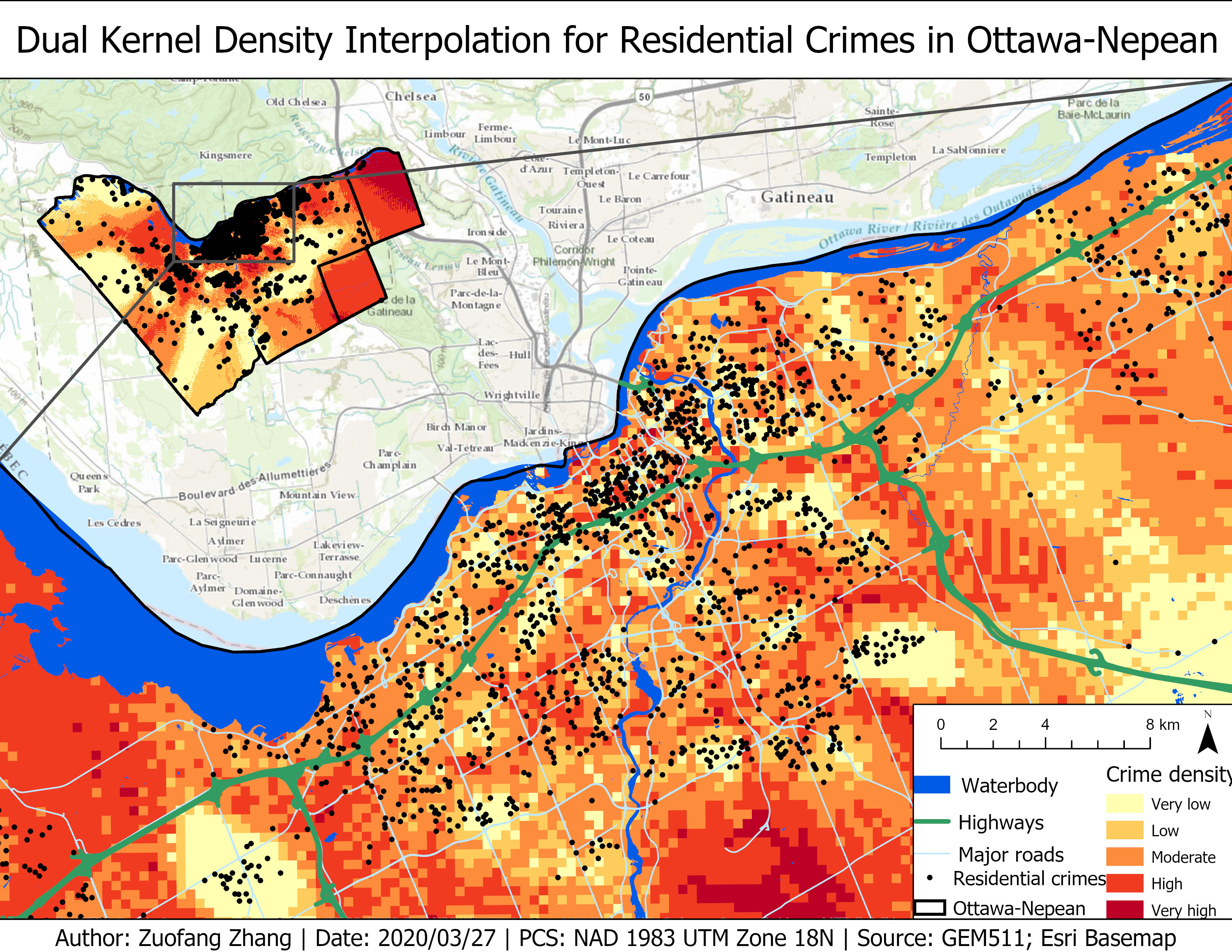
Fig.6 showed the residential crime density calculated using the dual kernel density analysis with the incident locations overlaid on the top of the interpolation surface. Darker red indicated higher crime density. Similar to the result of the single kernel density analysis, the center part of the city showed higher crime density. However, in contrast to the single kernel density result, the other high crime density clusters located in the eastern part of the Ottawa-Nepean region. The dual kernel density analysis included a population variable, while the single kernel density analysis only considered the crime observations. As a result, the dual kernel density result can better represent the reality by providing relative crime density estimations which were adjusted according to the population density.
Reference
CrimeStat documentation (n.d.) Retrieved on April 3, 2020 from https://www.icpsr.umich.edu/CrimeStat/download.html