Regression analysis studies the relationship between a set of independent variables and a dependent variable. Geographically Weighted Regression (GWR) is a linear regression that can be used to model relationships and processes that vary over space (Plant, 2012). Similar to the other linear models, GWR uses a set of independent variables to make predictions or study the relationships between dependent and independent variables. Unlike the other global models that make predictions for the whole study area using the same set of parameter coefficients, GWR is a localized model whose coefficients of parameters are ranges of values reflecting the data’s spatial heterogeneity (Plant, 2012).
In GWR, we assume that the relationship between each independent variables and the dependent variable is not constant across the study area (Plant, 2012). As a result, the weighting of each observation used to predict the value of a specific location varies over space (Plant, 2012). The closer observation will have more influence in estimating the parameters for the location point than observations farther away.
GWR is a type of hierarchical modeling whose observations are not independent of each other. The observations of hierarchical models can fall into clusters. Within each cluster, the observations have similar attributes. For example, in this project, we classify the whole Vancouver region into five clusters. The values of independent variables within each cluster share some similarities such as high average income and low percent of immigrants. The outputs of GWR are localized parameters that vary across space and can be mapped individually. We can also plot the local R2 on the individual coefficient maps to assess how well the model fits observations in different clusters.
Ordinary Least Squares (OLS) linear regression uses a set of independent variables to make predictions over the whole study area (Plant, 2012). OLS assumes that no spatial autocorrelation occurs and processes have no variation over space, therefore, it can be considered as a global model (Plant, 2012). If the independence assumption is not met, in other words, if the data exhibit spatial non-stationarity, the results of OLS would be incorrect because it does not take into account the influence of spatial clusters. Therefore, if the spatial data being examined is not constant over space, GWR could provide better predictions of the dependent variable by estimating local parameters.
We can first use OLS to determine and evaluate significant independent variables using forward or backward selection. After conducing spatial analysis such as Moran’s I and Geary’s c statistics to examine the presence of spatial autocorrelation, we can notice whether values of independent variables are constant or not. If there is spatial autocorrelation, individual observations are not independent with each other. As a result, GWR should be used instead to make better predictions.
In this project, we used both GLR and GWR to predict child’s language skills across Vancouver. Five independent variables were chosen for both models: ESL (a binary variable indicating whether English is the child’s second language or not), RecImmig (% of the recent immigrants in the neighborhood), Income1000 (the average income in the neighborhood divided by 1000), SOC_SC (an index reflecting the child’s social skills), and LoneParent (% of the neighborhood families that are lone parent). Table 1 shows the difference in model goodness of fit between GLR and GWR. For both AIC and R2, GWR had better performance with smaller AIC and larger R2. As shown in Table 2, GLR only had a single set of parameter coefficients over the whole study area whose values fell into the ranges of parameter coefficients of GWR.
Table 1 Comparison of regression goodness of fit between GLR and GWR.
| R2 | Adjusted R2 | AIC | |
| GLR | 0.3746 | 0.3734 | 22527.3204 |
| GWR | 0.4815 | 0.4361 | 22360.5500 |
Table 2 The GLR parameters and the ranges of the GWR parameters for each variable.
| Intercept | SOC_SC | ESL | LONEPARENT | RECIMMIG | INCOME1000 | |
| GLR | 22.866067 | 0.621941 | 5.451903 | -0.316155 | 0.067444 | 0.086723 |
| GWR | -49.6547-55.3374 | 0.440344-0.875059 | -2.18108-10.9939 | -1.79068-1.99519 | -0.212653-0.369193 | -0.371838-2.14084 |
By using the Spatially Constrained Multivariate Clustering tool, we grouped Enumeration Areas (EAs) into five neighborhoods based on Childcare (% of families that spend 30 or more hours on childcare), Fam4 (% of the neighborhood families that have four or more members), LoneParent, RecImmig, and Income (Fig.1). The five spatial clusters referred to East Vancouver, Granville Island, Downtown Vancouver, Vancouver West, and Kitsilano respectively. The observations within each neighborhood cluster shared certain similarities of the above five variables. For example, as shown in Fig.2, Granville Island had relatively lower value of Fam4 but higher Income and LoneParent, while East Vancouver had relatively lower income but higher Fam4 and LoneParent.
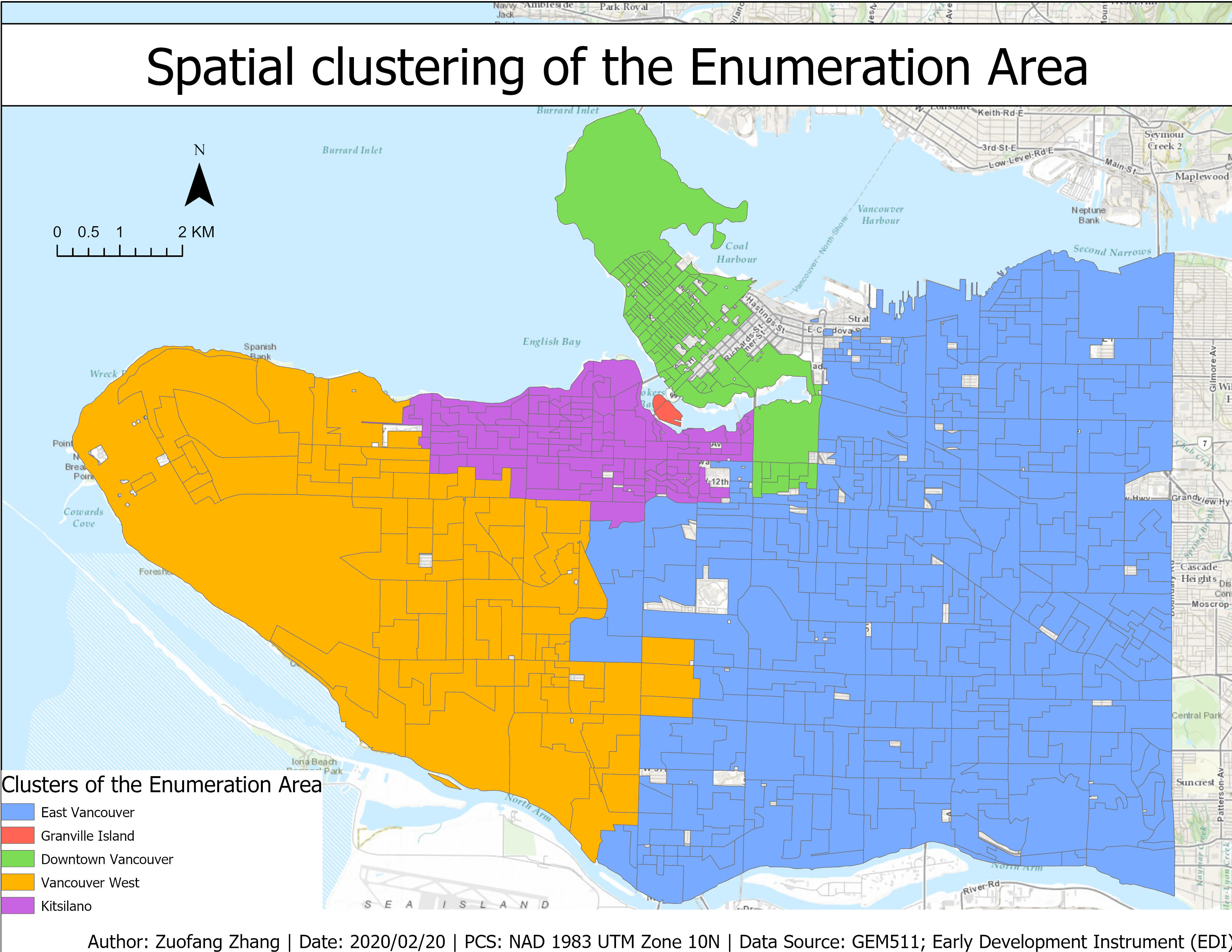
Fig.1 Spatial clustering of the Enumeration Area (EA) based on the following variables: the % of the families that spend 30 or more hours on childcare, the % of the neighborhood families that have 4 or more members, the % of the neighborhood families that are lone parent, the % of the neighborhood immigrants that are recent immigrants, the average income in the neighborhood.
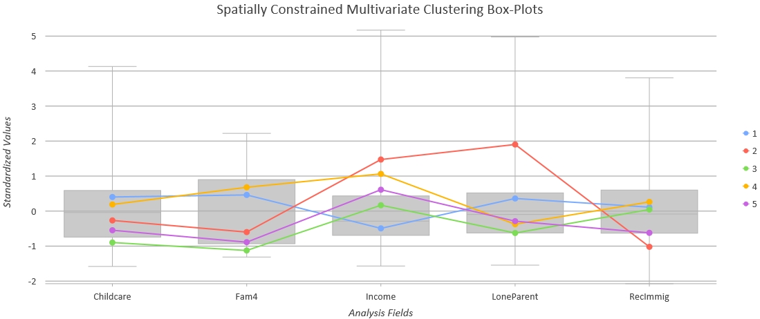
Fig.2 Spatially Constrained Multivariate Cluster Box-Plots. Cluster 1 to 5 represents five different neighborhoods which are East Vancouver, Granville Island, Downtown Vancouver, Vancouver West, and Kitsilano respectively.
Since the observations in Vancouver can be grouped into clusters, we concluded that the observations were not independent with each other and the data was non-stationary, as a result, the single set of parameters calculated from GLR cannot represent the relationship between child’s language skills and the independent variables very well. In contrast, GWR provided localized parameters that take into account spatial variation. For example, the coefficient of INCOME1000 calculated by GLR was 0.086723 which indicated that there was a positive relationship between the average neighborhood income and the child’s language skills. However, the positive regression was not always the truth as shown by the negative to positive range of the income parameter calculated by GWR (i.e., -0.371838-2.14084). In Fig.3, we can find that Vancouver West and Kitsilano as well as a part of East Vancouver showed a negative relationship between the income level and the child’s language skills. A unit increase in the average income was associated with a decrease in the child’s language skills. However, the highest positive value of income coefficient can also be observed in East Vancouver (Fig.3). This indicated that even within the same neighborhood, the relationship may be different. The box-plot showed that the average incomes in Vancouver West and Kitsilano were higher than East Vancouver. However, the % of families that spend more than 30 hours on childcare was higher in East Vancouver. The average income in Vancouver West and Kitsilano may have achieved the necessary requirements for children to develop their language skills. The increase in the income may associate with increased working time leading to less time for childcare which may negatively impact the child’s language skills. In contrast, children can benefit more from the increased average income in East Vancouver.
Fig.4 demonstrated the spatial distribution of the child’s social skill coefficient. Similar with the spatial distribution of the income coefficient, child’s social skills had larger impacts on the language skills in East Vancouver than the western part. A unit increase in social skills was associated with more increase in language skills of children in East Vancouver. However, unlike the income parameter, the social skill parameter had no negative impacts on language skills across the whole study region. As a result, we can conclude that better social skills were correlated with better language skills for all observations in Vancouver.
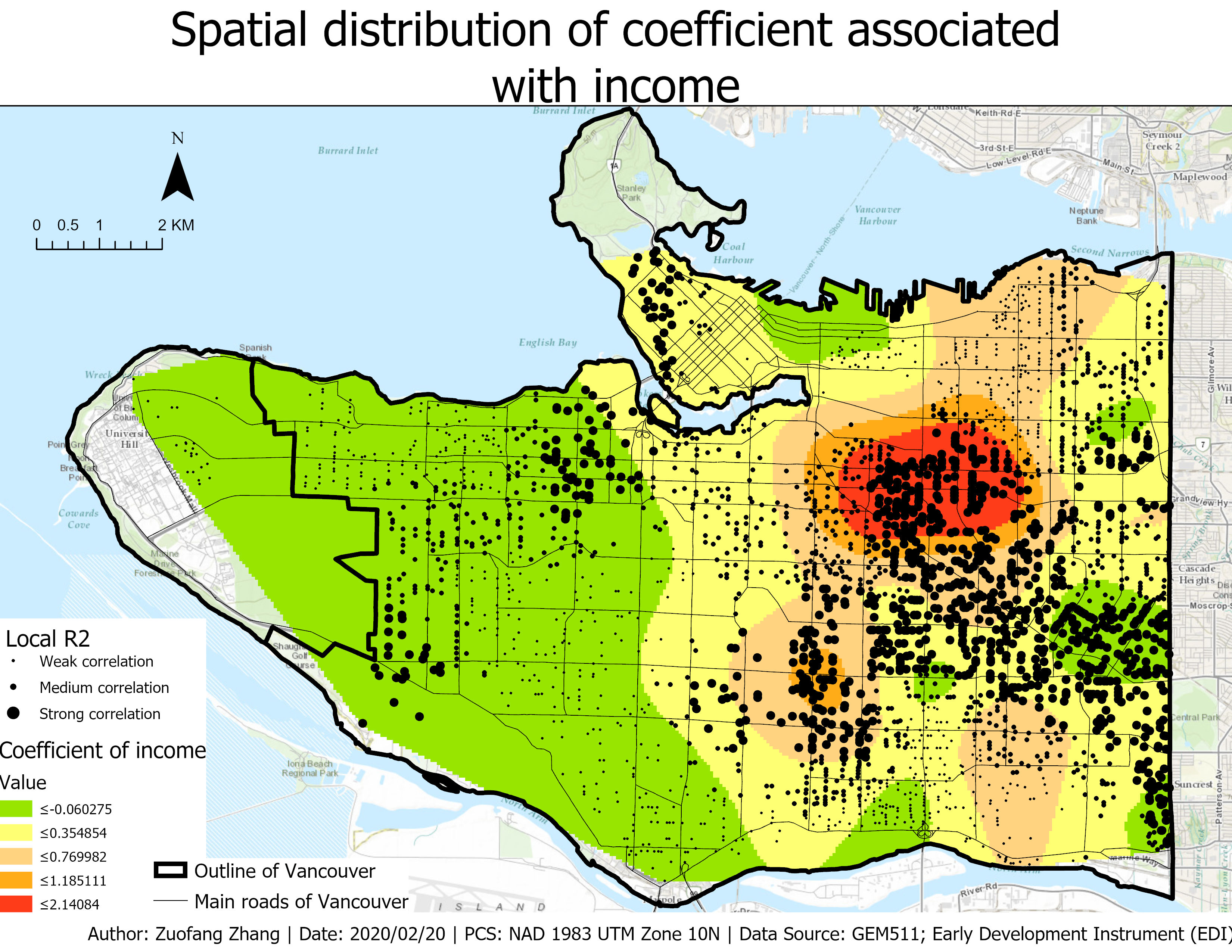
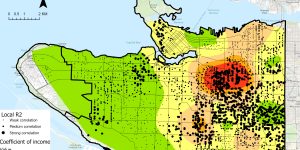
Fig.3 Spatial distribution of the coefficient associated with the average neighborhood income which is used to predict child’s language skills.
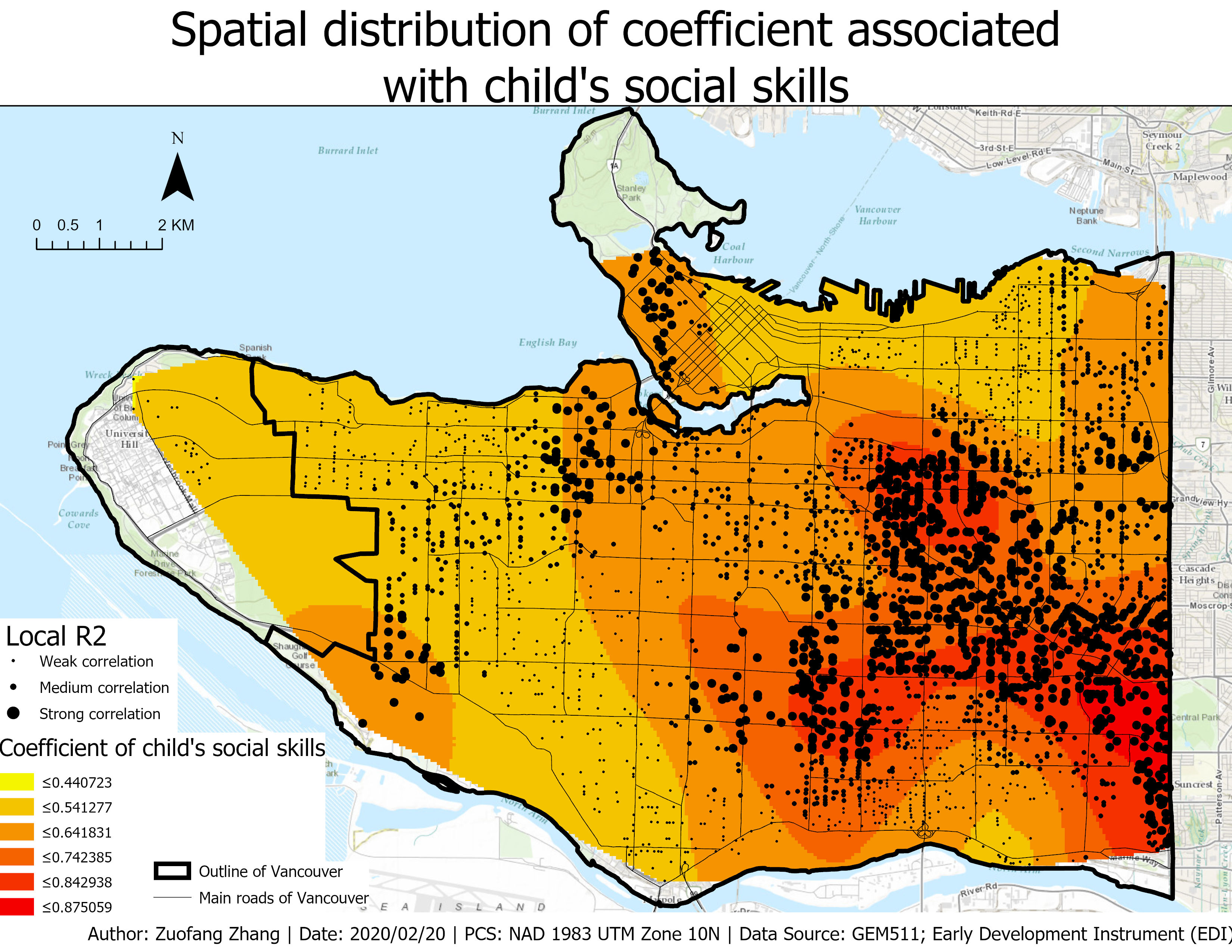
Fig.4 Spatial distribution of the coefficient associated with child’s social skills which is used to predict child’s language skills.
Since this is an observational study, no “cause and effect” can be made. If the observations were randomly selected, inference to the population can be made for Vancouver. Based on the local R2 plot, we can observe the goodness of fit variation across the whole study area. Local R2 values were grouped into three categories: weak, medium, and strong correlation. Generally, the correlation was stronger in East Vancouver compared to other clusters indicating that the model can better predict language skills in East Vancouver.
Reference
Plant, R. E. (2012). Spatial data analysis in ecology and agriculture using R. cRc Press.